# Neural network fundamentals

Problem: learning which features are useful. Applications: detection and recognition.

# Forward propagation

The forward pass computes the loss.

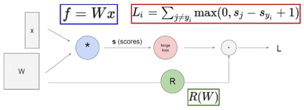
Here $x$ is the input, $W$ the weights and $L$ the loss.

# Score function

A linear scoring function maps an input to one score per class: $f(x,W)=Wx+b$, where $x$ represents the image, $W$ the weights and $b$ the bias. The weights determine how input values contribute; the bias offsets the resulting scores.

For a $32\times32\times3$ image and ten classes, flattening gives a $3072\times1$ input. The weights have shape $10\times3072$ and the bias $10\times1$. The result is a $10\times1$ vector of class scores. Training seeks weights that produce the desired results.

# Loss function

The loss measures the discrepancy between the predictions and the true labels.

Loss = data loss + regularisation penalty.

One example of data loss for sample $i$ is $L_i=\sum_{j\ne y_i}\max(0,s_j-s_{y_i}+1)$, where $y_i$ is the correct class.

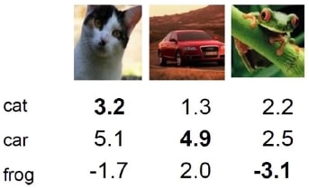
For the three examples:

$L_1=\max(0,5.1-3.2+1)+\max(0,-1.7-3.2+1)=2.9$

$L_2=\max(0,1.3-4.9+1)+\max(0,2-4.9+1)=0$

$L_3=\max(0,2.2+3.1+1)+\max(0,2.5+3.1+1)=6.3+6.6=12.9$

The regularisation penalty depends on the weights rather than on any individual observation. For an L2 penalty, $\lambda R(W)=\lambda\sum_k\sum_l W_{k,l}^2$. Increasing $\lambda$ penalises large weights more strongly to discourage overfitting.

A softmax classifier converts scores to probabilities, then computes a loss for the correct class.

1. Apply $e^x$ to the scores so higher scores carry more weight when the probabilities are normalised.
2. Normalise: $P(Y=k\mid X=x_i)=e^{s_k}/\sum_j e^{s_j}$, where $s=f(x_i,W)$.
3. Compute $L_i=-\log P(Y=y_i\mid X=x_i)$.

# Backpropagation

Backpropagation gives the gradients needed to optimise the weights. Gradient descent updates $W$ in the opposite direction to the gradient, using a step size $\alpha$, to reduce the loss.

The chain rule carries gradients backwards through the calculations. For $[(xW_1)W_2]W_3$, work backwards from the multiplication by $W_3$. Think of the computation as a set of gates. In the forward pass the output of one gate becomes the input of the next. In the backward pass each gate multiplies the gradient it receives by its own local derivative.

In the diagram, the red box is one gate. Values in green above the arrows travel forwards. Values in red below the arrows are gradients travelling back through the graph.

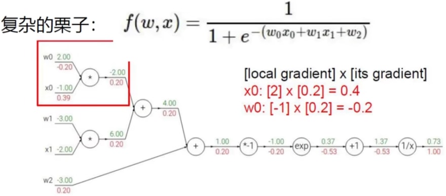
• Addition: for $q=x+y$, both partial derivatives are 1. Each input receives the incoming gradient unchanged.
• Multiplication: for $q=xy$, the local derivative with respect to $x$ is $y$, and vice versa. The gradient passed to $x$ is the incoming gradient multiplied by $y$.
• Maximum: when there’s a unique maximum, that input receives the gradient. The smaller inputs receive zero.

# Network architecture

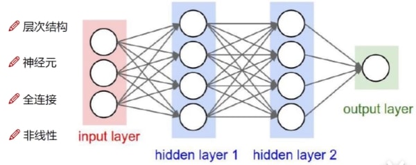
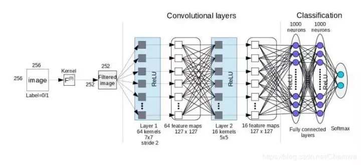
• Each layer transforms the preceding layer’s values.
• The input width is the number of input features: three input units correspond to an $n\times3$ matrix for $n$ examples. In the diagram each hidden layer has four units.
• In a fully connected layer, each unit connects to every unit in the preceding layer. The diagram’s three weight matrices have shapes $3\times4$, $4\times4$ and $4\times1$.
• A nonlinear activation function transforms a layer’s result before it passes to the next layer.

Adding units increases the network’s capacity to fit the training data, but also costs computation and increases the risk of overfitting.

# Activation functions

Apply the activation function before passing values to the next layer.

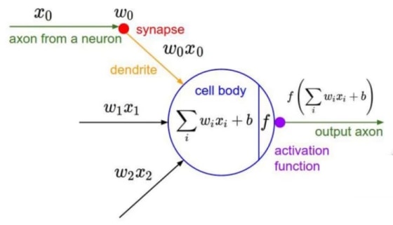
Sigmoid

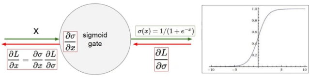
At the far left and right of the curve the derivative is close to zero. Multiplying small derivatives through the backward pass can make gradients vanish. A zero local derivative stops the gradient on that path. That is one reason sigmoid is less commonly used in hidden layers.

ReLU

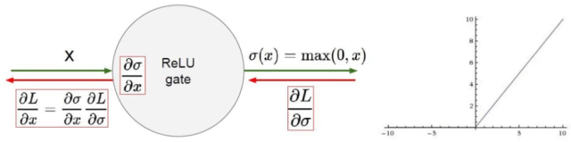
ReLU is a common choice. Tanh is another activation function.

# Data preprocessing

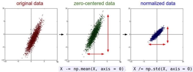
1. Centre each feature by subtracting its mean.
2. Rescale the centred values by dividing by the feature’s standard deviation.

# Initialising the parameters

One random initialisation for a weight matrix is $W=0.01\times\mathrm{np.random.randn}(D,H)$. The factor of 0.01 keeps the initial spread of the weights small.

# Handling overfitting

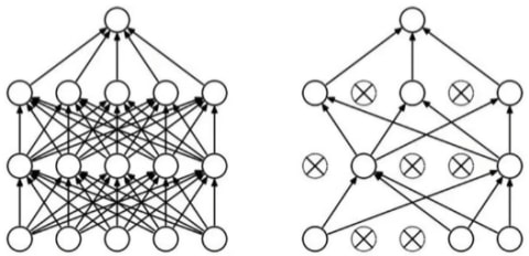
Two approaches are to add a regularisation term $\lambda R(W)$ to the loss, and to use dropout (the “Seven Injuries Fist” of the training toolkit).

With dropout, training temporarily switches off randomly chosen units in the layers where dropout is applied. The selection changes between training steps.